Numerical Algebraic Geometry: A Brief Introduction

My research focuses on numerical methods for solving systems of polynomial equations, making strong use of the geometric properties of algebraic sets. Here is a brief tasting to give an idea of what this means and what it can do.

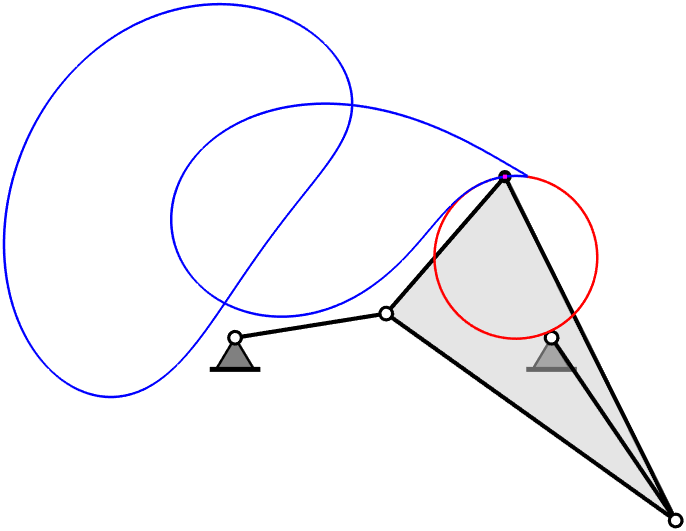
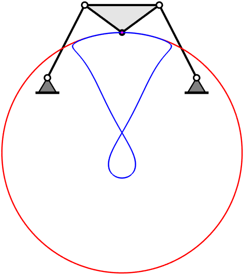
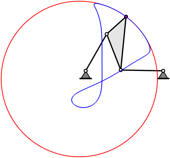
Many questions concerning how robots and other machines move, i.e., questions in kinematics, can be posed using polynomial equations. For example, the figure above shows a kind of robotic device called a Stewart-Gough platform. For general examples of such devices, one can generally calculate where the upper platform is located relative to the lower one knowing only the dimensions of all the parts. The problem can be stated as a system of seven quadratic polynomials that has at most 40 solution points. However, the particular example shown is a special case known as a Griffis-Duffy platform. This mechanism has a solution curve, as illustrated, which happens to be an algebraic curve of degree 40.

Numerical algebraic geometry solves such problems using homotopy to morph from an easy-to-solve initial problem to the potentially difficult target problem. The figures below illustrate a homotopy, \(h(z,t)\), between two cubic (degree 3) polynomials, \(f(z)\) and \(g(z)\):

\( h(z,t) = \gamma t g(z)+(1-t)f(z) = 0 \)

where \(\gamma\) is a random complex constant. (We'll see why it is there in a moment.) The homotopy is constructed so that at \(t=1\), \(h(z,1)=\gamma g(z)\), while at \(t=0\), \(h(z,0) = f(z)\). As \(t\) continuously varies from 1 to 0, the roots of \(h(z,t)\) follow paths from the roots of \(g\) to the roots of \(f\).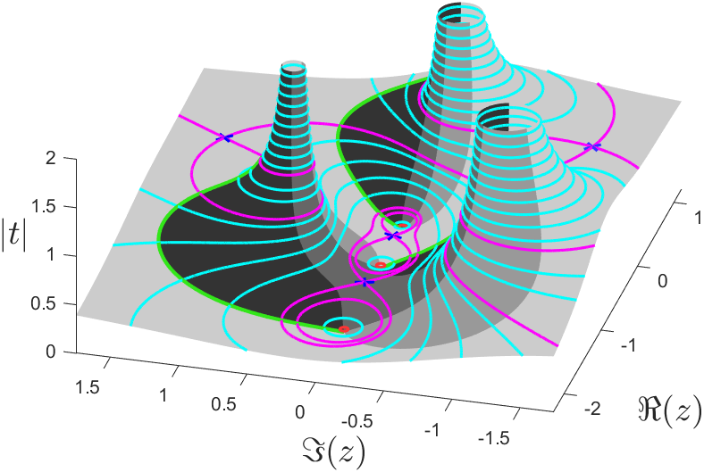

The idea is that if we want to compute the roots of a target polynomial \(f(z)\), we create a matching starting polynomial \(g(z)\) that is easy to solve and then track the solution paths from \(t=1\) to \(t=0\). The 2D picture above shows solution paths in green with an arrowhead indicating the direction of travel. They are smooth curves in the complex plane that are easy to track with numerical methods. Since \(f(z)\) and \(g(z)\) are cubics, i.e., degree 3, there are 3 paths, and their endpoints are the 3 solutions of \(f(z)=0\).

The real payoff in numerical algebraic geometry comes when the target f(z) is a complicated system of several polynomials in several variables, but for illustration we show just one variable here.

But how can we be sure the paths will be nice and will lead to all the roots of the target? The key to success is using complex numbers. (These are numbers of the form \(a+ib\), where \(i=\sqrt{-1}\).) We will only track paths as \(t\) moves on the real line, but for understanding why it works, let \(t\) take complex values. That is, let \(t=x+iy\in\mathbb{C}\). As both \(x\) and \(y\) vary, the roots of \(h(z,x+iy)=0\) form a surface like the one in the 3D view above. Each contour line on the surface consists of all the values of \(z\) for a constant value of \(|t|\), that is, the values of \(z\) as \(t\) goes around a circle centered on the origin in the complex plane. (In these plots, \(\Re(z)\) and \(\Im(z)\) are the real and imaginary parts of \(z\).) The roots of the target lie at the bottom of three depressions in the surface. For the homotopy method to succeed, we just need to ski downhill on this surface to reach these low points. In doing so, we must avoid hitting any saddle points (flat spots on the surface), because then it isn't clear which direction to go. You can see that the paths in the Top View (green with arrowhead) lie along the border between light gray and dark gray in the 3D picture. These paths steadily descend on the 3D surface.

There are a few contours (magenta curves) that cross themselves at the saddle points of this surface (blue x's). For success, all we have to do is make sure that none of the values of \(t\) that give saddle points are in the real interval \(0 < t \leq 1\). That's where the random \(\gamma\) comes into play. If we vary \(\gamma\), the \(z\)-coordinates of the saddle points stay the same, but the corresponding \(t\) values move. It can be shown that choosing \(\gamma\) randomly in the complex plane gives a zero chance of any saddle point lying on the real interval \(0 \lt t \leq 1\), and so the solution paths miss them, and the homotopy succeeds with probability 1.

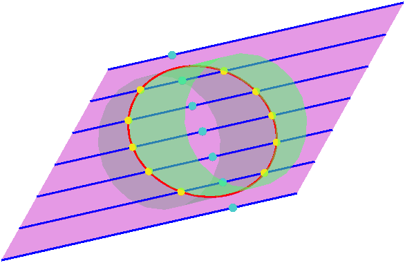
Numerical algebraic geometry is able to solve systems with higher-dimensional solutions sets, i.e., curves, surfaces, etc., that live in higher dimensional spaces. These are handled by slicing them down to reduce their dimension and projecting them to reduce the dimension of the space they live in. The figures below show a cylinder sliced down to an ellipse and a curve in space projected to a plane. Using random slices and projections preserves the degree and the irreducible factors of the original set.

To get an inkling of why geometry in higher dimensions is of practical interest, consider that a rigid body moving in our everyday three-dimensional space is formulated mathematically as a motion in a six-dimensional space called \(SE(3)\). (SE="special Euclidean"). It is 6-dimensional because the body can translate in 3 directions and rotate about 3 axes. In fact, it is often convenient to model \(SE(3)\) as a 6-dimensional hypersurface, the Study quadric, inside 7-dimensional projective space, \(\mathbb{P}^7\). Using that approach, the Stewart-Gough problem has 7 equations in 7 variables. In the image near the top of this page, the 3D curve traced by a point attached to the platform is an example of a projection: we are only seeing the translation of that point of the platform while we are ignoring how the orientation of the platform changes during motion along the curve.

It may be even more mind expanding to consider that we do all our calculations in the complex number field. So every variable has both a real and an imaginary part. This means that when one models \(SE(3)\) as a hypersurface in 7-complex-dimensional projective space, \(\mathbb{CP}^7\), the computations effectively occur in a 14-real-dimensional space.

For a deep dive, see my books on the Publications page.

For a quicker read, try:

C.W. Wampler and A.J. Sommese,
Numerical Algebraic Geometry and Algebraic Kinematics, (preprint)
Acta Numerica, 20:469--567, 2011. (doi)

An even more brief treatment, including a short discussion of the Griffis-Duffy platform illustrated above is:

A.J. Sommese, J. Verschelde, and C.W. Wampler,
Advances in Polynomial Continuation for Solving Problems in Kinematics, (preprint)
ASME Journal of Mechanical Design 126:2:262-268 (2004). (doi)

Some fun with planar curves

A straight-edge draws a line, and a compass draws a circle. These are algebraic curves of degree 1 and 2. Stepping up a notch in complexity, a four-bar linkage draws a degree 6 curve (a "sextic"), called a four-bar coupler curve. By adjusting the sizes of the links, one can obtain a wide variety of shapes. Engineers use this capability to design machines to perform specialized tasks, such as guiding how the wheels on a car react to bumps in the road so that the vehicle has good stability and handling.

At any point along a smooth curve in the plane, there exists an osculating circle that touches the curve with multiplicity 3. This gives us the definition of curvature. At special points along an algebraic curve, the osculating circle may touch with higher multiplicity, making the two curves hug each other even more closely. Excluding the case of a parallelogram (which draws complete circles), the highest possible multiplicity for contact between a circle and a four-bar coupler curve is 6. The figures below show several cases of this.

Given the four side lengths of a four-bar linkage, we can obtain various coupler curves by changing the other two sides of the coupler triangle. Using numerical algebraic geometry, we can find all pairs of coupler curves and circles that touch each other with multiplicity 6. For a general four-bar linkage, there are 72 such pairs, counting complex-valued ones. The number of real ones varies, depending on the lengths of the links. By computing all 72 solutions, we can be sure to find all the real ones.

For more, see:

C.W. Wampler, M. Husty, and J.D. Hauenstein,
Sixth-order singularities of the 3RR planar pentad mechanism, (preprint)
3rd IMA Conference on Mathematics of Robotics, Sep. 24-26, 2025.

A curve in 3-space

A free-floating rigid body in 3-dimensional space has 6 degrees of freedom: it can translate independently in the 3 coordinate directions, and it can rotate independently about those directions as well. (See the discussion of \(SE(3)\) above.) However, if we constrain some point of the body to lie on a surface or on a curve, the body is no longer free-floating; it moves on a subspace of \(SE(3)\).

The figure below shows a rigid body consisting of four rods, each terminating in a ball. The centers of two balls are constrained to follow lines, and the center of a third ball is constrained to a plane. The body still has one degree of freedom of motion. The figure shows the path the fourth ball follows during this motion.

Constraining a point to lie on a line is equivalent to constraining it to lie on two planes whose intersection is that line. Accordingly, the illustrated scenario is a case of a rigid body subjected to 5 point-to-plane constraints, which is one of the scenarios treated in the reference below. Since each point-to-plane constraint removes 1 degree of freedom, we see that the rigid body has 1 remaining degree of freedom: \(6-5=1\). In other words, the body has a motion curve.

Numerical algebraic geometry applies whenever one wishes to solve systems of polynomials, not just ones deriving from the kinematics of mechanisms. But kinematics is a rich source of such problems, with the advantage for the purpose of illustration of having concrete visual representations.

For a paper about point-to-plane constraints see:

C.W. Wampler,
On a rigid body subject to point-plane constraints, (preprint)
ASME J. of Mechanical Design, 128(1):151--158, Jan. 2006. (doi)